Today we are going to customize a simple boxplot by overlaying individual data points.

Note that there’s a few pieces of code lying around on the UCLA website, but we are going to proceed in a different way. Note also that stripplot offers a lot of functionality, including a variation of the idea discussed here. And the built-in dotplot command comes close to what we would like to do, except that it is not a twoway command.

First, we need a dataset. Let’s consider, for example, the dataset physed which is used in the [MV] manual (it is also discussed in the Stata Journal). It is described as follows:

You have measured the flexibility, speed, and strength of the 80 students in your physical education class. You want to split the class into four groups, based on their physical attributes, so that they can receive the mix of flexibility, strength, and speed training that will best help them improve.

There are 4 variables and we are interested in describing the distribution of the three numerical variables, independent of group membership. You may recall that a boxplot summarizes the distribution of a continuous variable by using a 5-point summary, much like tabstat or other tables of statistics can do in the results window.

Here are a few steps before we can go on with displays of basic boxplots:

webuse physed
local j = 1
foreach v of varlist flexibility-strength {
  rename `v' value`j'
  local ++j
}
gen id = _n
reshape long value, i(id) j(variable)
label define variable 1 "flexibility" 2 "speed" 3 "strength"
label values variable variable

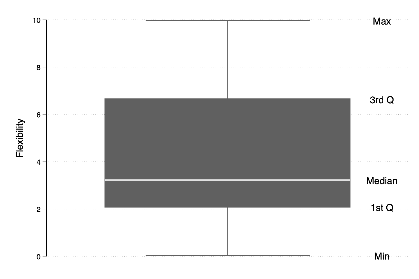
Now that we have data in long format (so that we can process all numerical data at once), here is a simple reminder of what a boxplot is:

summarize value if variable == 1, detail
graph box value if variable == 1, text(`r(p50)' 95 "Median") ///
  text(`r(p25)' 95 "1st Q") text(`r(p75)' 95 "3rd Q") ///
  text(`r(min)' 95 "Min") text(`r(max)' 95 "Max") ///
  ytitle("Flexibility")

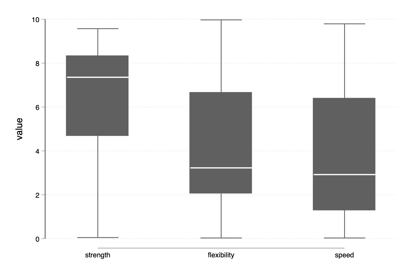
With all three variables, the command simply becomes:

graph box value, over(variable, sort(1) descending)

Unfortunately, graph (h)box is not a member of the twoway family so it is not possible to overlay a scatterplot or a dotplot on top (or beneath). However, we don’t necessarily need the box, and as suggested by Tufte a simpler version might just be used to highlight the median and draw whiskers around it. I wrote a scrappy R function to build such lightweight boxplot a long ago. Hence, we can simply draw all the elements we need one after the other.

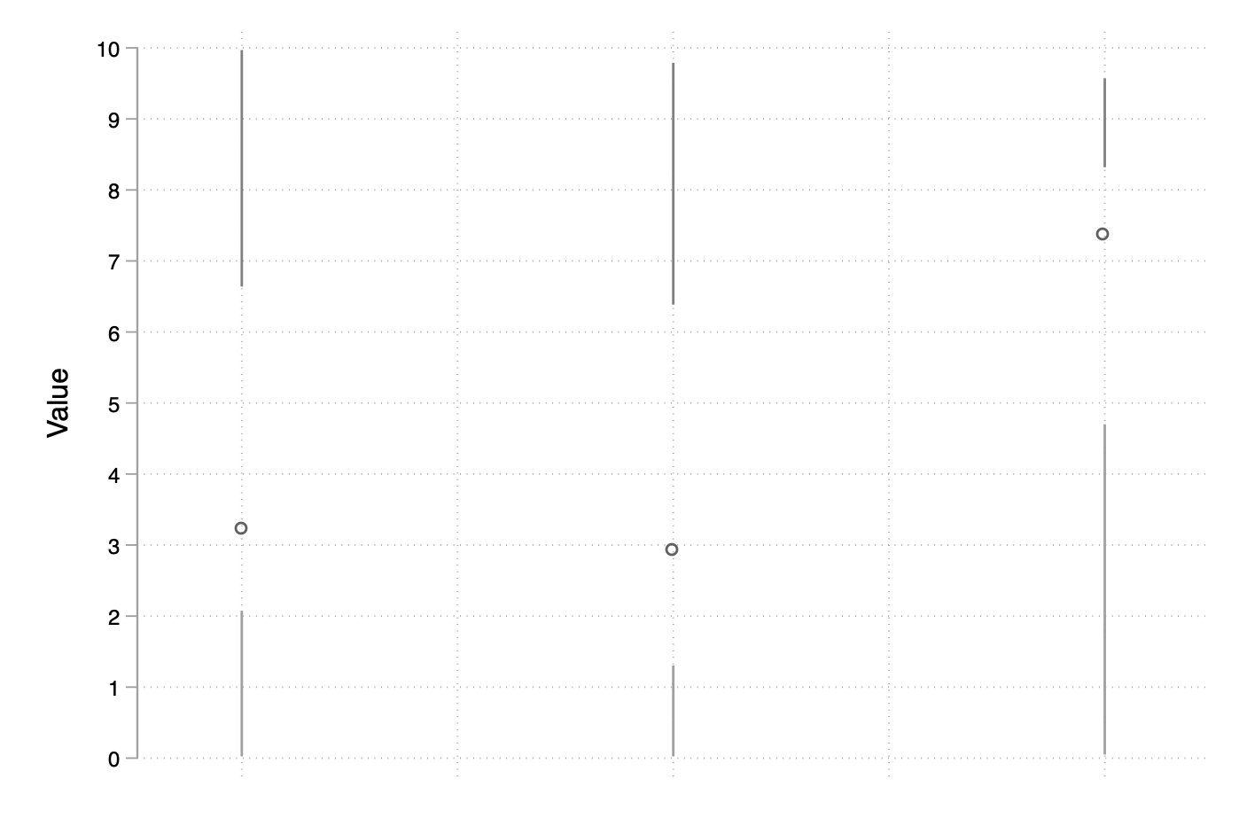
Let’s look at a simplified version the classical boxplot without drawing proper wiskers and “outside” value. Our whiskers will simply extend from the 1st or 3rd quartile to the minimum and maximum values, respectively:

preserve
collapse (min) lo=value (p25) q1=value (p50) q2=value (p75) q3=value (max) hi=value, by(variable)
twoway (scatter q2 variable, ylab(0(1)10) xscale(r(0.8 3.2) off fill) xlab(,nolabels) ytitle("Value") xtitle("")) ///
  (rspike q1 lo variable) (rspike hi q3 variable), legend(off)

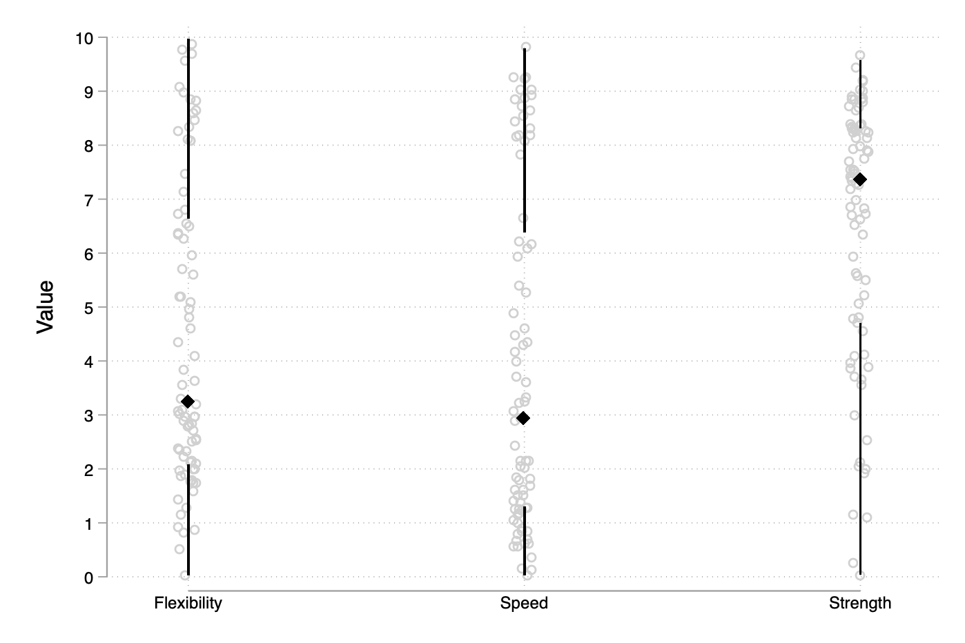
Next, we could add the datapoints with an additional call to scatter but the dataset we are currently working is no longer available because of collapse and it would probably more cumbersome to save it and merge it afterwards (especially given the fact that there won’t exist a common id variable). Let’s just append the aggregate statistics like we would do with window functions:

by variable, sort: egen hi = max(value)
by variable, sort: egen lo = min(value)
by variable, sort: egen q1 = pctile(value), p(25)
by variable, sort: egen q3 = pctile(value), p(75)
by variable, sort: egen q2 = median(value)
label define variable 1 "Flexibility" 2 "Speed" 3 "Strength", modify
twoway (scatter value variable, jitter(3) mcolor(gs13)) (scatter q2 variable, ms(d) msize(medium) mcol(black)) ///
  (rspike q1 lo variable, lcol(black)) (rspike hi q3 variable, lcol(black)), ///
  ylab(0(1)10) xscale(r(0.8 3.2)) xlab(1/3, valuelabel noticks) ytitle("Value") xtitle("") legend(off)

This looks like a lot of typing but it is not difficult to wrap the above code into a proper command. Likewise it would not require too much of an effort to apply Tukey’s rules for defining “outside” values and to update how whiskers do extend around the 1st and 3rd quartiles.