Here is an implementation of the Newton-Raphson algorithm in Racket Scheme.

Our goal is to implement a toy example of logistic regression, where the parameters of the statistical model are estimated using Newton-Raphson iterative algorithm. This approach basically looks like this in R: (For more details, please refer to the following blog post: Write your own logistic regression function in R.)

log_reg <- function(X, y) {
  beta <- rep.int(0, ncol(X))
  for (i in seq_len(100)) {
    b_old <- beta
    alpha <- X %*% beta
    p <- 1 / (1 + exp(-alpha))
    W <- as.numeric(p * (1 - p))
    XtX <- crossprod(X, diag(W) %*% X)
    score <- t(X) %*% (y - p)
    delta <- solve(XtX, score)
    beta <- beta + delta
  }
  return(beta)
}

The Newton algorithm belongs to root finding methods, and it is usually employed with a univariate function, $f$, for which we want to find, say, its zeros or its maximum. In the above case, we seek the maximum of a given function–this is maximum likelihood theory after all. Recall that when we want to find an approximate root of $f(x)=0$, we usually start with a guess, say $x_n$, and we approximate $f(x)$ by its tangent line $f(x_n)+f'(x_n)(x-x_n)$. This is basically how Newton’s method looks like, and this yields an improved guess, $x_{n+1}=x_n-\frac{f(x_n)}{f'(x_n)}$, based on the root found for the tangent.¹ It is pretty straightforward to write a little recursive solution to this problem, e.g. in Racket:

;; f(x) = x^2 - 9
(define (f x) (- (sqr x) 9))

;; f'(x) = 2x
(define (fp x) (* 2 x))

;; increase tolerance (1e-6) if you want more accurate answer
(define (newton x f fp)
  (let ((guess (- x (/ (f x) (fp x)))))
    (if (> (abs (- x guess)) 1e-6)
      (newton guess f fp)
      guess)))

(display (newton 0.1 f fp))

Now, suppose we are interested in finding the maximum of a given function, $f(x)$. Let us assume that $f'$ is continuously differentiable, and that $f''(x^{\star})\neq 0$, with $x^{\star}$ the root we are looking for. Maximizing $f$ amounts to find the root of $f'(x)$, which is depicted in the next picture, and at each step we will approximate $f'(x^{\star})$ with the linear Taylor expansion $f'(x^{\star})\approx f'(x^{(t)}) + \left(x^{\star}-x^{(t)}\right)f''(x^{(t)})$ ($=0$).

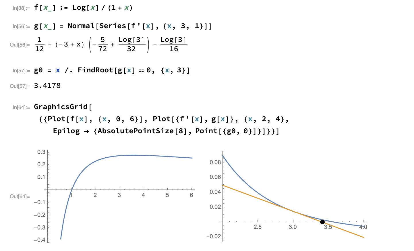
As can be seen, the derivative $f'$ is approximated by its tangent at $x^{(t)}$, so that we will approximate its root by the root of the tangent line (highlighted as a black dot in the above picture). Hence, we have:

$$ x^{\star} = x^{(t)} - \frac{f'(x^{(t)})}{f''(x^{(t)})} = x^{(t)} + h^{(t)}, $$

where $h^{(t)}$ is a refinement to the current guess at step $t$, $x^{(t)}$. The updating equation for Newton-Raphson is then simply $x^{(t+1)}=x^{(t)}+h^{(t)}$, which is the very last line in the for loop in the R function above. (I don’t know why the authors used the temporary variable b_old, BTW.) Note that $h^{(t)} = -\frac{f'(x^{(t)}}{f''(x^{(t)}}$. In this particular case, this optimization problem amounts to find the MLE $\hat\theta$, where $\theta$ is the parameter of interest in the statistical model, and $f$ is the likelihood function.² It can be shown that the Newton’s method has quadratic convergence, which means that the precision of the solution will usually double with each iteration.³

The logistic model can be written as $\log\left(\frac{p}{1-p}\right) = \beta_0 + \beta_1X_1+\beta_2X_2$, for two fixed predictors $X_1$ and $X_2$. Individual probabilities $p_i$ ($i=1,\dots,n$) are a function of both the vectors $x_i$ and $\beta$, and as formulated above, the model implies that $p_i=\frac{\exp(x_i^T\beta)}{1+\exp(x_i^T\beta)}$. It can be shown that the likelihood reads:

$$ \ell(\beta) = \sum_{i=1}^n\left\{ y_i(x_i^T\beta) - \log\left(1+\exp(x_i^T\beta)\right) \right\}, $$

and to maximize this likelihood function we need to compute the score function—this is the variable score in the R code—which is the derivative of $\ell$ with respect to $\beta$ parameters (in this example, we only considered two predictors):

$$ \frac{\partial\ell}{\partial\beta} = \begin{bmatrix}\frac{\partial\ell}{\partial\beta_0} \cr \frac{\partial\ell}{\partial\beta_1} \cr \frac{\partial\ell}{\partial\beta_2} \end{bmatrix} = \underbrace{\boldsymbol{X}^T(y-\boldsymbol{p})}_{\texttt{t(X) %*% (y - p)}}. $$

We also need the second derivative, $\frac{\partial^2\ell}{\partial\beta_j\partial\beta_k}$, which can be written:

$$ \frac{\partial}{\partial\beta_k}\frac{\partial\ell(\beta)}{\partial\beta_j} = \sum_{i=1}^n\left\{x_{ij}\left(y_i-\frac{\partial p_i(x_i,\beta)}{\partial\beta_k}\right) \right\}. $$

In matrix notation, we would write $\frac{\partial^2\ell}{\partial\beta^2} = -\boldsymbol{X}^T\boldsymbol{W}\boldsymbol{X}$ (see also the blog cited at the beginning of the post), where $\boldsymbol{W}$ is an $n$-by-$n$ diagnoal matrix where the $i$-th diagonal element equals $p_i(1-p_i)$, whence the code XtX <- crossprod(X, diag(W) %*% X).

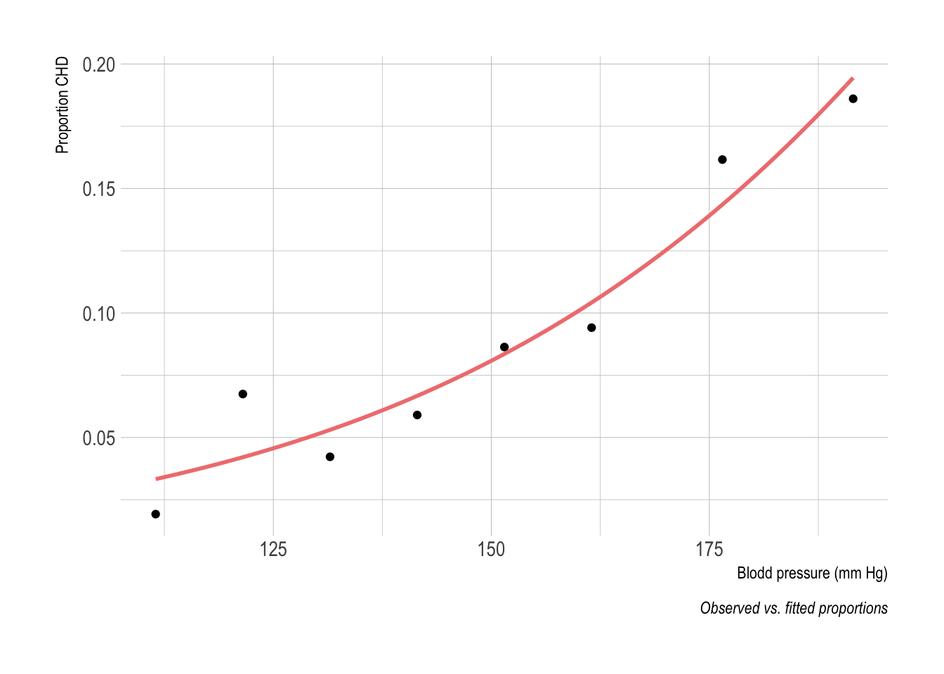
In the end, we would like to estimate the parameters of the logistic model fitted to the dataset shown below (observed and fitted values; see handout 3 in the rstats-biostats project for R code and a brief description of the data):

Other than basic mathematical operators and functions, the most important piece of code we need is an equivalent of crossprod, the matrix cross-product, and solve, which is used to solve a system of equations. Luckily, both procedures are available in racket/math. The instructions inside the R loop could thus be translated literally using untyped Racket as follows:

#lang racket
(require math/matrix)

;; data definition
(define beta (col-matrix [0 0]))
(define y (col-matrix [0.01923077 0.06746032 0.04225352 0.05904059
                       0.08633094 0.09411765 0.16161616 0.18604651]))
(define X (matrix [[1 1 1 1 1 1 1 1]
                   [111.5 121.5 131.5 141.5 151.5 161.5 176.5 191.5]]))
(define alpha (matrix* (matrix-transpose X) beta))

;; helper functions
(define (logit x) (/ 1 (+ 1 (exp (- x)))))
(define (complement x) (- 1 x))

;; scoring matrix
(define p (matrix-map logit alpha))
(define W (matrix-map * p (matrix-map complement p)))
(define XtX (matrix* X (matrix* (diagonal-matrix (matrix->list W))
                                                 (matrix-transpose X))))
(define score (matrix* X (matrix-map - y p)))
(define delta (matrix-solve XtX score))

This code yields exactly the same results as a first pass in the R loop of log_reg. Given how easy it is to go from a for loop to recursive function calls, these five steps can easily be wrapped into a proper function using local let* bindings. Note that there exist various converters that help to go from list or vector to matrix that we could use instead, and more importantly, there is even a data frame package (developped by Alex Harsányi) which could further simplifies all the data mockup.

And that’s it! An interesting alternative would be to implement the EM algorithm for logistic regression, proposed by Scott and Sun.